Tutorial 3: Electron Energy Loss Spectroscopy
In this third tutorial, we will learn how to calculate the Electron Energy Loss Spectrsocopy (EELS) using TDDFT.
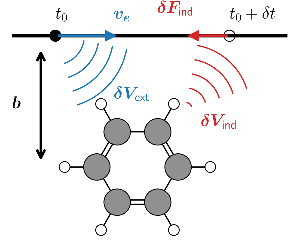
During EELS, a charged particle (typically an electron), is passing in the vinicity of a molecule. The electric field generated by the moving charge excite the system which will then create an induced electric field.
One of the advantage of electronic excitation is the possibility to excite so call dark mode that can not be excited via light. For more details on the method, you can refer to the chapter 6 of [Barbry2018thesis]
Requirements: Have executed tutorial 2
Initialize TDDFT
As stated in the requirements, you must have executed the tutorial 2 before to start this tutorial. Otherwise, the DFT inputs will not be present.
It is a good practice when running EELS calculations to check that the electron trajectory do not intersect any atom before to start calculations.
We will start then by loading the deometry of the systems (file
siesta.xyz) using ASE, and define the trajectory of the electron.
import numpy as np
import ase.io as io

atoms = io.read("siesta.xyz")
velec = np.array([0.0, 75.0, 0.0])
beam_offset = np.array([0.0, 0.0, 5.0])
Another condition to keep in mind is that the beam_offset (the b
arrow on the top diagram) must be perpendicular to the electron
trajectory defined by the electron velocity vector velec, i.e.,
velec.dot(beam_offset) == 0.0.
The function pynao.tddft_tem.check_collision check that all these
conditions are respected.
from pynao.tddft_tem import check_collision

print(atoms.positions.shape)
check_collision(velec, beam_offset, atoms.positions)
(5, 3)
pynao.tddft_tem => tem parameters:
vdir:  [0. 1. 0.]
vnorm:  75.0
beam_offset:  [0. 0. 5.]
We can then initialize the TDDFT calculations in the same fashion than in tutorial 2.
from pynao import tddft_iter

td = tddft_iter(label="siesta")
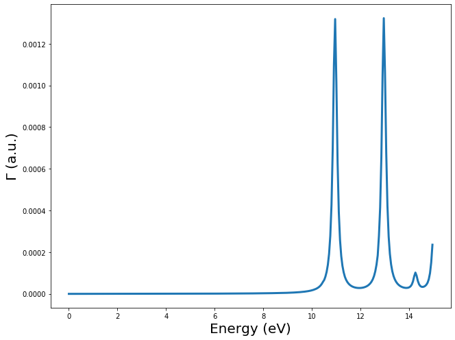
Once the kernel has been calculated, we can calculate the EELS spectra
of the molecule by calling the method get_EELS_spectrum. This method
takes three main inputs:
freq: the frequencies at which to calculate the spectra. The frequencies must be given in Hartree.velec: the velocity vector of the charged particle in atomic units. 100 keV \(\sim\) 75.0 a.u.beam offset: the shift of the beam trajectory. must be perpendicular tovelec
from ase.units import Ha

freq = np.arange(0.0, 15.0, 0.05)/Ha
Vext, EELS = td.get_EELS_spectrum(freq, velec=velec, beam_offset=beam_offset)
Total number of iterations: 1943
import matplotlib.pyplot as plt

h = 7
w = 4*h/3
ft = 20

fig = plt.figure(1, figsize=(w, h))
ax = fig.add_subplot(111)
ax.plot(freq*Ha, EELS.imag, linewidth=3)
ax.set_xlabel(r"Energy (eV)", fontsize=ft)
ax.set_ylabel(r"$\Gamma$ (a.u.)", fontsize=ft)
fig.tight_layout()
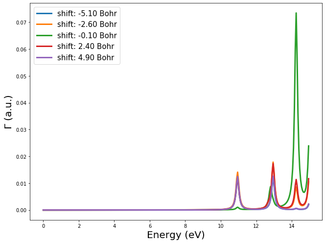
One can easily run sevral trajectories in a for loop by changing the electron velocity vector or the beam offset
shifts = np.arange(-5.1, 5.5, 2.5)
velec = np.array([0.0, 25.0, 0.0])

gammas = []
for i, sh in enumerate(shifts):
    offset = np.array([0.0, 0.0, sh])
    Vext, EELS = td.get_EELS_spectrum(freq, velec=velec, beam_offset=offset)
    gammas.append(EELS)
Total number of iterations:  7963
Total number of iterations:  10087
Total number of iterations:  12172
Total number of iterations:  14295
Total number of iterations:  16305
fig = plt.figure(2, figsize=(w, h))
ax = fig.add_subplot(111)

for i, sh in enumerate(shifts):
    ax.plot(freq*Ha, gammas[i].imag, linewidth=3, label="shift: {0:.2f} Bohr".format(sh))
ax.set_xlabel(r"Energy (eV)", fontsize=ft)
ax.set_ylabel(r"$\Gamma$ (a.u.)", fontsize=ft)
ax.legend(fontsize=ft-5)
fig.tight_layout()