Tutorial 1: calculate the polarizability of CH4 molecule with PySCF
In this first tutorial, we will learn how to calculate the polarizability of a molecule using time dependent density functional theory (TDDFT). In this tutorial, PySCF will be used to perform the ground state calculations.
Requirements: have PyNAO and PySCF installed
Run DFT via PySCF
We assume that you already were able to install PyNAO and therefore PySCF program (since PySCF is required to use PyNAO).
Before to run DFT calculations, we need to run first DFT calculations, in this tutorial, we will use PySCF
Notes: Siesta can be used as well to run DFT calculations, but it must be installed first. Runing PyNAO for Siesta DFT calculations will be covered in tutorial 2
The first step is to define the geometry, PySCF requires to enter the greometry in a string of the form
Symbol x, y, z;
You can easily create such string in Python.
CH4_geometry = """C  0.00000000, 0.00000000, 0.00000000;
H  0.62911800, 0.62911800, 0.62911800;
H  -0.62911800, -0.62911800, 0.62911800;
H  0.62911800, -0.62911800, -0.62911800;
H  -0.62911800, 0.62911800, -0.62911800;"""
We can now launch DFT calculation with PySCF via the following lines
from pyscf import gto, scf

mol = gto.M(atom=CH4_geometry, basis='ccpvdz', spin=0)
gto_mf = scf.UHF(mol)
gto_mf.kernel()
converged SCF energy = -40.1987085424816 <S^2> = 3.2329694e-13 2S+1 = 1
-40.198708542481626
Run TDDFT with PyNAO
Now that DFT calculations are terminated we can start to launch TDDFT
calculations. The first step is to initialize the system and calculate
the kernel by calling tddft_iter.
This method takes the DFT inputs, in this case the varaibles gto_mf
and mol obtained from PySCF calculations.
from pynao import tddft_iter

td = tddft_iter(mf=gto_mf, gto=mol)
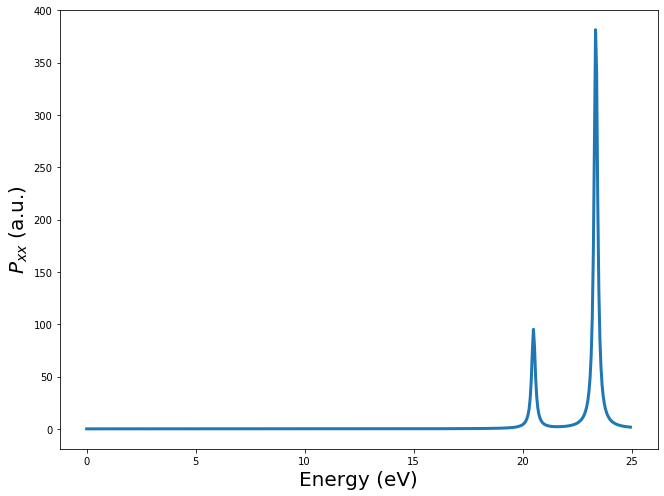
Once the kernel has been calculated, we can calculate the polarizability
of the molecule by calling the method comp_polariz_inter_Edir.
This method tkes two main inputs:
freq: the frequencies at which to calculate the polarizability. It must be a complex number, the real part is the actual frequencies points, while the imaginary part is the actual broadening of the polarizability. In general it will betddft_iter.eps. The frequencies must be given in Hartree.Edir: the direction of the external electric field
import numpy as np
import scipy.constants as cte

Ha = cte.physical_constants["Hartree energy in eV"][0]

freq = np.arange(0.0, 25.0, 0.05)/Ha + 1j * td.eps
p_mat = td.comp_polariz_inter_Edir(freq, Eext=np.array([1.0, 1.0, 1.0]))
Total number of iterations: 9918
import matplotlib.pyplot as plt

h = 7
w = 4*h/3
ft = 20

fig = plt.figure(1, figsize=(w, h))
ax = fig.add_subplot(111)
ax.plot(freq.real*Ha, -p_mat[0,0, :].imag, linewidth=3)
ax.set_xlabel(r"Energy (eV)", fontsize=ft)
ax.set_ylabel(r"$P_{xx}$ (a.u.)", fontsize=ft)
fig.tight_layout()