Advanced tutorial: TDDFT with Silver cluster
In this tutorial, we will see how to calculate the polarizability of a silver cluster of 147 atoms using TDDFT method.
In this folder you should find the following files
siesta.fdf: the siesta input file to run DFT calculation.geometry.siesta.fdf: The geometry of the system for siesta.Ags147.xyz: The geometry of the system in xyz format. The ghost atoms are represented as normal silver atoms.Ag.psf: pseudopotential for silver atomsAgs.psf: pseudopotential for ghost atoms
The inputs files can be downloaded from this link
Run Siesta calculations
The first step is to launch siesta calculation to get the inputs for
TDDFT. This can be done by (assuming siesta executable is in your
PATH)
siesta < siesta.fdf > siesta.out
To run directly from the notebook, you need to add ! before the call
as shown n the cell below.
!siesta < siesta.fdf > siesta.out
Run TDDFT calculations
Sytem initialization
Once Siesta calculation finished, we have all the necessary inputs to launch the TDDFT calculations. We first need to initialize the system.
PyNAO must be able to find inputs from siesta, this can be done by
setting the parameter label. It must be the same than the value
SystemLabel found in siesta.fdf. The directory for the
calculation is given by the parameter cd.
Other parameters are optional, the most important ones are
krylov_solver: the Krylov solver type used for solving the linear system of equationkrylov_options: The options for the solver. A tolerance of10e-5is often enough to get accurate results.level: To control the number of radial and angular grids (see`pyscf.dft.Grids<http://pyscf.org/pyscf/dft.html?highlight=grids#pyscf.dft.gen_grid.Grids>`__)krylov_solver: Iterative solver to use to solve the linear system of equation see SciPy pagekrylov_options: The options for the Krylov solveriter_broadening: The broadening applied to the polarizability. The broadening should not be smaller than \(\frac{3}{2}d\omega\), where \(d\omega\) is the frequency step.
import os
import numpy as np

from ase.units import Ry, eV, Ha
from pynao import tddft_iter

# Run TDDFT
dname = os.getcwd()

# Calculate the kernel
eps = 0.15
td = tddft_iter(label='siesta', cd=dname, verbosity=4, krylov_solver="lgmres",
                krylov_options={"tol": 1.0e-5, "atol": 1.0e-5},
                iter_broadening=eps/Ha, tol_loc=1e-4, tol_biloc=1e-6, jcutoff=7,
                xc_code='LDA,PZ', level=0, GPU=True)
pynao.mf            ====> self.pseudo:  True
pynao.mf            ====> Number of orbitals:  2853
pynao.prod_basis    ====> Time for call vrtx_cc_batch: 5.82 sec, npairs: 12350
pynao.prod_basis    ====> libnao.vrtx_cc_batch is done!
pynao.prod_basis    ====> Time after vrtx_cc_batch:  294.69 sec
pynao.prod_basis    ====>libnao.get_vrtx_cc_batch is calling
pynao.mf            ====> Number of dominant and atom-centered products (91137, 12939)
spin 0: block_size: (512, 1024); grid_size: (2, 13)
pynao.tddft_iter    ====> self.xc_code: LDA,PZ
Rough calculations of the polarizability
We can now calculate the polarizability of the system. In this example we will
First do a rough calculation to get a approximation to the excitation over a braod frequency range
calculate for a fewer frequencies a more accurate solution around the excitation peak.
The aim is to reduce the amount of total iteration necessary to define the surface dipole mode.
# Reduce the tolerance for faster convergence (at the price of accuracy)
td.krylov_options["tol"] = 1.0e-3
td.krylov_options["atol"] = 1.0e-3

freq = np.arange(0.0, 10.0, 0.2)/Ha + 1.0j*td.eps
p_mat = td.comp_polariz_inter_Edir(freq, Eext=np.array([1.0, 0.0, 0.0]), tmp_fname="pol.tmp")
dir: 0, iw: 0/50; w: 0.0000;nite: 11; time: 10.859995042999799
dir: 0, iw: 1/50; w: 0.2000;nite: 11; time: 9.78481567199924
dir: 0, iw: 2/50; w: 0.4000;nite: 11; time: 9.944984920999559
dir: 0, iw: 3/50; w: 0.6000;nite: 11; time: 9.735718634998193
dir: 0, iw: 4/50; w: 0.8000;nite: 11; time: 9.6907503370021
dir: 0, iw: 5/50; w: 1.0000;nite: 12; time: 10.587485121999634
dir: 0, iw: 6/50; w: 1.2000;nite: 12; time: 10.600325448998774
dir: 0, iw: 7/50; w: 1.4000;nite: 12; time: 10.624163034000958
dir: 0, iw: 8/50; w: 1.6000;nite: 13; time: 11.515673274996516
dir: 0, iw: 9/50; w: 1.8000;nite: 13; time: 11.524202458000218
dir: 0, iw: 10/50; w: 2.0000;nite: 13; time: 11.608784874995763
dir: 0, iw: 11/50; w: 2.2000;nite: 13; time: 11.566674744994089
dir: 0, iw: 12/50; w: 2.4000;nite: 14; time: 12.421578346999013
dir: 0, iw: 13/50; w: 2.6000;nite: 14; time: 12.402781926997704
dir: 0, iw: 14/50; w: 2.8000;nite: 15; time: 13.34854932899907
dir: 0, iw: 15/50; w: 3.0000;nite: 14; time: 12.575863885002036
dir: 0, iw: 16/50; w: 3.2000;nite: 15; time: 13.342396928994276
dir: 0, iw: 17/50; w: 3.4000;nite: 17; time: 15.082635270002356
dir: 0, iw: 18/50; w: 3.6000;nite: 15; time: 13.320954039998469
dir: 0, iw: 19/50; w: 3.8000;nite: 14; time: 12.362988486995164
dir: 0, iw: 20/50; w: 4.0000;nite: 13; time: 11.45963800699974
dir: 0, iw: 21/50; w: 4.2000;nite: 13; time: 11.489849892997881
dir: 0, iw: 22/50; w: 4.4000;nite: 12; time: 10.596434751001652
dir: 0, iw: 23/50; w: 4.6000;nite: 12; time: 10.608972675996483
dir: 0, iw: 24/50; w: 4.8000;nite: 11; time: 9.759126446006121
dir: 0, iw: 25/50; w: 5.0000;nite: 12; time: 10.619216213002801
dir: 0, iw: 26/50; w: 5.2000;nite: 13; time: 11.552363629001775
dir: 0, iw: 27/50; w: 5.4000;nite: 13; time: 11.573655088002852
dir: 0, iw: 28/50; w: 5.6000;nite: 13; time: 11.559512362997339
dir: 0, iw: 29/50; w: 5.8000;nite: 13; time: 11.594928004000394
dir: 0, iw: 30/50; w: 6.0000;nite: 13; time: 11.559449200998642
dir: 0, iw: 31/50; w: 6.2000;nite: 13; time: 11.56299164799566
dir: 0, iw: 32/50; w: 6.4000;nite: 13; time: 11.637743485000101
dir: 0, iw: 33/50; w: 6.6000;nite: 14; time: 12.483829980999872
dir: 0, iw: 34/50; w: 6.8000;nite: 14; time: 12.496328995002841
dir: 0, iw: 35/50; w: 7.0000;nite: 13; time: 11.608795957996335
dir: 0, iw: 36/50; w: 7.2000;nite: 14; time: 12.50216210900544
dir: 0, iw: 37/50; w: 7.4000;nite: 13; time: 11.63096589199995
dir: 0, iw: 38/50; w: 7.6000;nite: 13; time: 11.582422439001675
dir: 0, iw: 39/50; w: 7.8000;nite: 13; time: 11.565565188000619
dir: 0, iw: 40/50; w: 8.0000;nite: 12; time: 10.666582566002035
dir: 0, iw: 41/50; w: 8.2000;nite: 11; time: 9.773726674997306
dir: 0, iw: 42/50; w: 8.4000;nite: 12; time: 10.681150926997361
dir: 0, iw: 43/50; w: 8.6000;nite: 11; time: 9.783439842998632
dir: 0, iw: 44/50; w: 8.8000;nite: 11; time: 9.780670565000037
dir: 0, iw: 45/50; w: 9.0000;nite: 11; time: 9.770246159001545
dir: 0, iw: 46/50; w: 9.2000;nite: 11; time: 9.778547871996125
dir: 0, iw: 47/50; w: 9.4000;nite: 11; time: 9.764264632998675
dir: 0, iw: 48/50; w: 9.6000;nite: 10; time: 8.86918604800303
dir: 0, iw: 49/50; w: 9.8000;nite: 11; time: 9.770509477995802
Total number of iterations:  630
We can analyze the rough polarizability obtained
import matplotlib.pyplot as plt

np.save("freq_range_rough.npy", freq.real)
np.save("polarizability_inter_rough.npy", p_mat)

iw = np.argmax(-p_mat[0, 0, :].imag)
print("max(Pxx) = {}".format(freq.real[iw]*Ha))

h = 9
w = 4*h/3
ft = 20
lw = 4

fig = plt.figure(1, figsize=(w, h))
ax = fig.add_subplot(111)

ax.plot(freq.real*Ha, -p_mat[0, 0, :].imag, linewidth=lw)
ax.set_xlabel(r"Energy (eV)", fontsize=ft)
ax.set_ylabel(r"$P_{xx}$ (a.u.)", fontsize=ft)
plt.show()
max(Pxx) = 3.4000000000000004
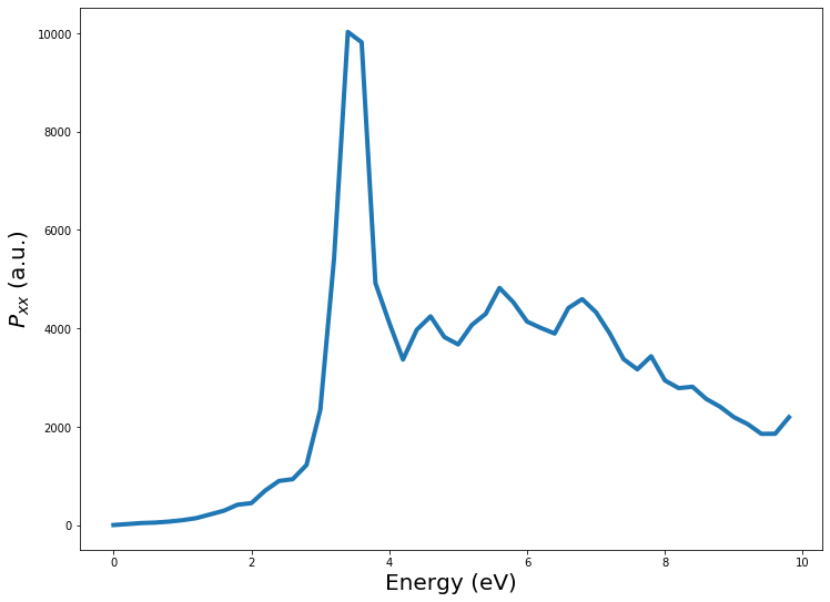
We see from the graph of \(P_{xx}\) is aroung 3.5 eV.
Accurate calculation of the excitation peak
We can now do more accurate calculations on a reduced frequency range (between 3.3 and 3.7 eV) with a higher tolerance for the iterative solver.
td.krylov_options["tol"] = 1.0e-5
td.krylov_options["atol"] = 1.0e-5

freq2 = np.arange(3.3, 3.7, 0.01)/Ha + 1.0j*td.eps
p_mat2 = td.comp_polariz_inter_Edir(freq2, Eext=np.array([1.0, 0.0, 0.0]), tmp_fname="pol.tmp")
dir: 0, iw: 0/41; w: 3.3000;nite: 27; time: 24.13607315299305
dir: 0, iw: 1/41; w: 3.3100;nite: 27; time: 23.969823163999536
dir: 0, iw: 2/41; w: 3.3200;nite: 27; time: 23.999744434993772
dir: 0, iw: 3/41; w: 3.3300;nite: 27; time: 23.965296750997368
dir: 0, iw: 4/41; w: 3.3400;nite: 27; time: 23.975718581001274
dir: 0, iw: 5/41; w: 3.3500;nite: 27; time: 23.95826233200205
dir: 0, iw: 6/41; w: 3.3600;nite: 27; time: 23.99717613199755
dir: 0, iw: 7/41; w: 3.3700;nite: 27; time: 24.083581273000163
dir: 0, iw: 8/41; w: 3.3800;nite: 27; time: 24.133442885002296
dir: 0, iw: 9/41; w: 3.3900;nite: 27; time: 24.194143676002568
dir: 0, iw: 10/41; w: 3.4000;nite: 27; time: 24.769432850996964
dir: 0, iw: 11/41; w: 3.4100;nite: 27; time: 24.14564469600009
dir: 0, iw: 12/41; w: 3.4200;nite: 27; time: 24.070358536999265
dir: 0, iw: 13/41; w: 3.4300;nite: 27; time: 24.21153749199584
dir: 0, iw: 14/41; w: 3.4400;nite: 27; time: 24.191062513004
dir: 0, iw: 15/41; w: 3.4500;nite: 27; time: 24.45884982500138
dir: 0, iw: 16/41; w: 3.4600;nite: 27; time: 24.443401043994527
dir: 0, iw: 17/41; w: 3.4700;nite: 27; time: 24.531622656002583
dir: 0, iw: 18/41; w: 3.4800;nite: 26; time: 23.579618449002737
dir: 0, iw: 19/41; w: 3.4900;nite: 26; time: 23.601201855002728
dir: 0, iw: 20/41; w: 3.5000;nite: 26; time: 23.555409278997104
dir: 0, iw: 21/41; w: 3.5100;nite: 26; time: 23.674540478998097
dir: 0, iw: 22/41; w: 3.5200;nite: 26; time: 23.477661156000977
dir: 0, iw: 23/41; w: 3.5300;nite: 26; time: 23.426061420002952
dir: 0, iw: 24/41; w: 3.5400;nite: 26; time: 23.364886967996426
dir: 0, iw: 25/41; w: 3.5500;nite: 25; time: 22.487443521000387
dir: 0, iw: 26/41; w: 3.5600;nite: 25; time: 22.47092411099584
dir: 0, iw: 27/41; w: 3.5700;nite: 25; time: 22.471652000996983
dir: 0, iw: 28/41; w: 3.5800;nite: 24; time: 21.535540573000617
dir: 0, iw: 29/41; w: 3.5900;nite: 24; time: 21.642063125000277
dir: 0, iw: 30/41; w: 3.6000;nite: 24; time: 21.62391388099786
dir: 0, iw: 31/41; w: 3.6100;nite: 24; time: 21.705278376000933
dir: 0, iw: 32/41; w: 3.6200;nite: 23; time: 20.624220448000415
dir: 0, iw: 33/41; w: 3.6300;nite: 23; time: 20.66294245699828
dir: 0, iw: 34/41; w: 3.6400;nite: 23; time: 20.55991561400151
dir: 0, iw: 35/41; w: 3.6500;nite: 23; time: 20.895650813996326
dir: 0, iw: 36/41; w: 3.6600;nite: 23; time: 20.965098015003605
dir: 0, iw: 37/41; w: 3.6700;nite: 23; time: 20.74679407399526
dir: 0, iw: 38/41; w: 3.6800;nite: 23; time: 20.875799485002062
dir: 0, iw: 39/41; w: 3.6900;nite: 23; time: 21.27209885999764
dir: 0, iw: 40/41; w: 3.7000;nite: 23; time: 21.496940359997097
Total number of iterations:  1676
np.save("freq_range_acc.npy", freq2.real)
np.save("polarizability_inter_acc.npy", p_mat2)

iw = np.argmax(-p_mat2[0, 0, :].imag)
print("max(Pxx) = {}".format(freq2.real[iw]*Ha))

fig = plt.figure(2, figsize=(w, h))
ax = fig.add_subplot(111)
ax.plot(freq.real*Ha, -p_mat[0, 0, :].imag, linewidth=lw)
ax.plot(freq2.real*Ha, -p_mat2[0, 0, :].imag, linewidth=lw)
ax.set_xlabel(r"Energy (eV)", fontsize=ft)
ax.set_ylabel(r"$P_{xx}$ (a.u.)", fontsize=ft)

plt.show()
max(Pxx) = 3.509999999999995
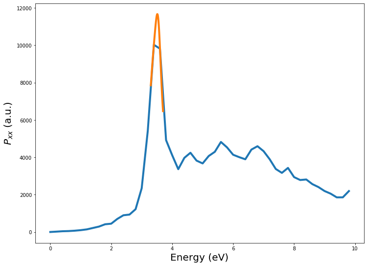
Now we have a much more accurate description of the surface dipole peak, which is located at 3.51 eV.
Electronic density change
Lets calculate the electronic density change distribution \(\delta n\) in space to vizualize the surface dipole.
from ase.units import Bohr
from pynao.m_comp_spatial_distributions import spatial_distribution

# From `siesta.out` we can get the box size
# siesta: Automatic unit cell vectors (Ang):
# siesta:   30.214756    0.000000    0.000000
# siesta:    0.000000   30.214756    0.000000
# siesta:    0.000000    0.000000   30.214756

box = np.array([[-16.0, 16.0],
                [-16.0, 16.0],
                [-16.0, 16.0]])/Bohr


dr = np.array([0.3, 0.3, 0.3])/Bohr

# initialize spatial calculations
# see file `pynao.m_comp_spatial_distributions` for some description of the inputs
# be aware that the density change in product basis, nao_td.dn could be loaded
# from file, allowing you to change the spatial density distribution parameters
# without redoing the full calculation
# One mus also be careful to the inputs of `spatial_distribution`
# they must be the same the the function used to calculate `td.dn`
spd = spatial_distribution(td.dn, freq2, box, dr=dr, label="siesta",
                           excitation="light",cd=dname, verbosity=4,
                           tol_loc=1e-4, tol_biloc=1e-6, jcutoff=7,
                           level=0)

# compute spatial density change distribution at a specific frequency
w0 = 3.51/Ha
spd.get_spatial_density(w0)

np.save("dn_iter_spatial.npy", spd.dn_spatial)
pynao.mf            ====> self.pseudo:  True
pynao.mf            ====> Number of orbitals:  2853
pynao.prod_basis    ====> Time for call vrtx_cc_batch: 5.47 sec, npairs: 12350
pynao.prod_basis    ====> libnao.vrtx_cc_batch is done!
pynao.prod_basis    ====> Time after vrtx_cc_batch:  289.83 sec
pynao.prod_basis    ====>libnao.get_vrtx_cc_batch is calling
pynao.mf            ====> Number of dominant and atom-centered products (91137, 12939)
fig2 = plt.figure(2, figsize=(w, h))
ax = fig2.add_subplot(111)

idx = 54 # middle of the system
vmax = np.max(abs(spd.dn_spatial[:, :, 54].imag))
vmin = -vmax
ext = [box[0, 0], box[0, 1], box[1, 0], box[1, 1]]
ax.imshow(spd.dn_spatial[:, :, 54].imag, cmap="seismic", vmin=vmin, vmax=vmax, interpolation="bicubic", origin="lower", extent=ext)
plt.show()
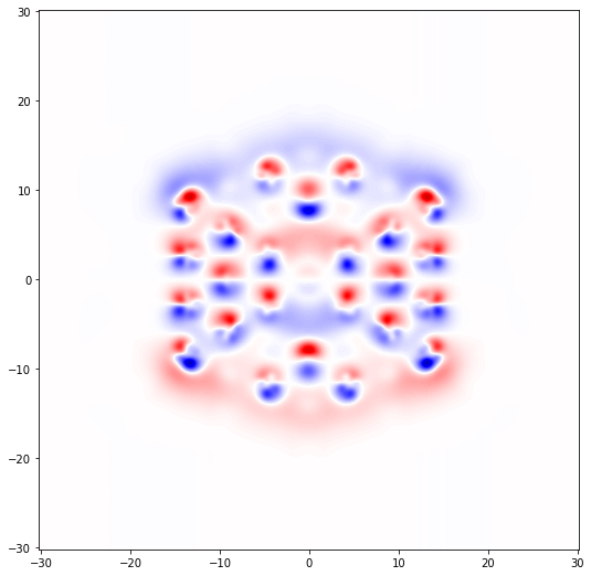
The surface plasmon is clearly visible at the cluster surface. We can also see very well the density change created by the d-electron of the silver clusters.
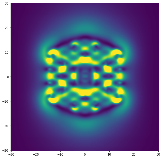
Lets now calculate the distribution of the electric field enhancement.
## compute Efield
Efield = spd.comp_induce_field()
np.save("Efield_tem_spatial.npy", Efield)

## compute intensity
intensity = spd.comp_intensity_Efield(Efield)
np.save("Efield_intensity_tem_spatial.npy", intensity)
fig3 = plt.figure(3, figsize=(w, h))
ax = fig3.add_subplot(111)

vmax = np.max(abs(intensity[:, :, 54]))
vmin = 0.0
print(vmin, vmax)
ax.imshow(intensity[:, :, 54], vmin=vmin, vmax=vmax/3, interpolation="bicubic", origin="lower", extent=ext)
plt.show()
0.0 13.022563