Tutorial 2: calculate the polarizability of CH4 molecule with Siesta

In this second tutorial, we will learn how to calculate the polarizability of a molecule using TDDFT as in tutorial 1. However in this case, we will use Siesta for the DFT calculations.

Requirements: have PyNAO, PySCF and Siesta installed

Run DFT with Siesta

We assume here that Siesta is properly installed and configured on your system. We will assume also that siesta executable as been added to your PATH

Method 1: run Siesta via the command line

The first way to run Siesta is to call the executable from the command line. For this, you should make sure to

to have a siesta fdf input file on the disk
to have the necessary pseudopotential in the folder

First, we will define the siesta.fdf file (we already included the pseudopotential files in the folder). In the siesta.fdf file

take note of the SystemLabel variable, you will need it for PyNAO
the option COOP.Write must be set to True
the option XML.Write must be set to True

Let write the siesta.fdf file to disk

siestafdf = """SystemName      siesta
SystemLabel     siesta

COOP.Write      True
DM.MixingWeight 0.01
DM.NumberPulay  4
DM.Tolerance    0.0001
MD.MaxForceTol  0.02    eV/Ang
MD.NumCGsteps   0
MaxSCFIterations        10000
PAO.BasisType   split
SCFMustConverge False
WriteCoorXmol   True
WriteDenchar    True
XML.Write       True

Spin            non-polarized
XC.functional   GGA
XC.authors      PBE

MeshCutoff      3401.4232530459053      eV
PAO.EnergyShift 0.025   eV

NumberOfSpecies 2
NumberOfAtoms   5
%block ChemicalSpecieslabel
    1 6 C
    2 1 H
%endblock ChemicalSpecieslabel

%block PAO.BasisSizes
    C     DZP
    H     DZP
%endblock PAO.BasisSizes

AtomicCoordinatesFormat  Ang
%block AtomicCoordinatesAndAtomicSpecies
     0.000000000      0.000000000      0.000000000 1
     0.629118000      0.629118000      0.629118000 2
    -0.629118000     -0.629118000      0.629118000 2
     0.629118000     -0.629118000     -0.629118000 2
    -0.629118000      0.629118000     -0.629118000 2
%endblock AtomicCoordinatesAndAtomicSpecies
"""

with open("siesta.fdf", "w") as fl:
    fl.write(siestafdf)

We can now launch DFT calculation with Siesta via the command line

!siesta <siesta.fdf > siesta.out

Method 2: run Siesta via ASE

The Atomic Simulation Environment (ASE) provides all an environment to run atomistic calculations. It is possible to run Siesta calculations via ASE, which is more friendly than running Siesta from the command line.

The advantage of using ASE is that you do not need to write the siesta fdf input file by hand, and you don’t need to copy the pseudopotentials. However, make sure that the ASE Siesta calculator is properly setup.

from ase.calculators.siesta import Siesta
from ase.units import eV, Ry

# First we need to build the molecule
# It can be done directly via ASE
from ase.build import molecule
atoms = molecule('CH4')

# Or you can load the molecule geometry from file
#import ase.io as io
#atoms = io.read(fname)

# set-up the Siesta parameters
siesta = Siesta(
      mesh_cutoff=250*Ry,
      basis_set='DZP',
      pseudo_qualifier='gga',
      xc="PBE",
      energy_shift=(25 * 10**-3) * eV,
      fdf_arguments={
        'SCFMustConverge': False,
        'COOP.Write': True,
        'WriteDenchar': True,
        'PAO.BasisType': 'split',
        'DM.Tolerance': 1e-4,
        'DM.MixingWeight': 0.01,
        "MD.NumCGsteps": 0,
        "MD.MaxForceTol": (0.02, "eV/Ang"),
        'MaxSCFIterations': 10000,
        'DM.NumberPulay': 4,
        'XML.Write': True,
        "WriteCoorXmol": True})

atoms.set_calculator(siesta)

# Run Siesta calculation
e = atoms.get_potential_energy()
print("DFT potential energy", e)

Run TDDFT with PyNAO

Now we can run TDDFT calculations similarly to what was done in tutorial 1 with PySCF.

The first step is to initialize the system and calculate the kernel by calling tddft_iter.

For Siesta inputs, we need to call tddft_iter with the label parameter. It must be the same label than the one indicated by SystemLabel in the Siesta fdf file.

from pynao import tddft_iter

td = tddft_iter(label="siesta")

Once the kernel has been calculated, we can calculate the polarizability of the molecule by calling the method comp_polariz_inter_Edir.

This method takes two main inputs:

freq: the frequencies at which to calculate the polarizability. It must be a complex number, the real part is the actual frequencies points, while the imaginary part is the actual broadening of the polarizability. In general it will be tddft_iter.eps. The frequencies must be given in Hartree.
Edir: the direction of the external electric field

import numpy as np
from ase.units import Ha

freq = np.arange(0.0, 25.0, 0.05)/Ha + 1j * td.eps
p_mat = td.comp_polariz_inter_Edir(freq, Eext=np.array([1.0, 1.0, 1.0]))

Total number of iterations:  10853

import matplotlib.pyplot as plt

h = 7
w = 4*h/3
ft = 20

fig = plt.figure(1, figsize=(w, h))
ax = fig.add_subplot(111)
ax.plot(freq.real*Ha, -p_mat[0,0, :].imag, linewidth=3)
ax.set_xlabel(r"Energy (eV)", fontsize=ft)
ax.set_ylabel(r"$P_{xx}$ (a.u.)", fontsize=ft)
fig.tight_layout()

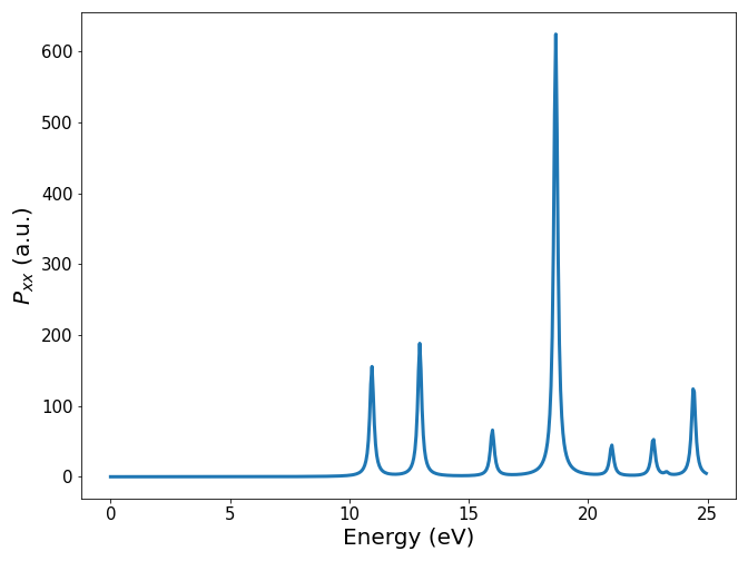
Remark

If you compare the spectra obtained in tutorial 1 and tutorial 2, you will see a quite different spectra, while the system is the same. Since the TDDFT part remained inchanged, it demonstrates how crucial is the quality of the DFT inputs in order to obtain reliable results.

The purpose of these tutorial is to demonstrate how to use PyNAO with PySCF and Siesta. It is the responsability of the user to ensure the quality of the calculations he is running.