GW Approximation and its implementation in PyNAO
Theory - Formalism
The GW approximation (GWA) has been shown to be a reliable method in order to obtain quasiparticle (QP) energies as well as many other physical properties of materials. Correspondingly, its formalism has been extensively presented in detail elsewhere. In particular, we refer users to read the recent paper of Koval P. et al. [koval2019GW] which extensively describes the implementation of \(G_0W_0\) calculations in MBPT_LCAO package.
Hamiltonian
In principle, GWA is derived from Many Body Perturbation Theory (MBPT) [Fetter1971]. The Green’s function theory is a proper way to investigate single-particle excitation QP energies [galitskii1958], [aryasetiawan1998gw]. Accordingly, the generalized Hedin’s GW formulation starts with the interacting Green’s function \(G_{\sigma}(\omega)\) which can be obtained in spectral representation as follows
where \(\psi_{i\sigma }\) and \(E_{i\sigma}\) represent some single-particle wavefunction and eigenenergy for each spin channel (\(\sigma = \uparrow , \downarrow\)). The quantities \(\eta\), and \(\varepsilon_{F}\) are a positive infinitesimal shift from the real axis and Fermi energy, respectively. The physical interpretation of the poles of \(G(\omega)\) in the prior equation is the exact QP energies for a charged system, i.e. \(N\pm1\) particles when QP will be particularly referred to an excitation stemming from the single-particle state [martin_GW_2016], [aryasetiawan1998gw]. Around Fermi level, \(\psi_{i\sigma}\) are the solutions of the following QP equation
where \(E_{i\sigma}\) represents a complex value of QP energy defining QP intensity and its lifetime given by \(1/Im(E_{i\sigma}(\omega)\). \(\Sigma_{\sigma} (r,r^{'},\omega)\) is the spin-resolved nonlocal complex potential known as the self-energy that arises from a first-order perturbation. In fact, all electron-electron interaction effects beyond non-interacting particles (Hartree potential) are included in the self-energy [Fetter1971], [Mattuck1976].
Self-energy and Screened interaction
Calculating the self-energy had remained a significant problem in condensed matter physics for decades. In 1965, Hedin formulated a set of coupled integral equations that determines a self-consistent relationship among the self-energy (\(\Sigma\)), the single-particle Green’s function, and the generalized screened Coulomb interaction (\(W\)) [hedin1965new]. Correspondingly, the spin-resolved matrix element of \(\Sigma_{\sigma}\) is given by integral equation including the interacting single-particle Green’s function \(G_{\sigma}(r,r^{'}; \omega)\) and \(W\) in space-spin-time coordinates when the product is a convolution in the frequency domain
Note that the imaginary part in the exponent term originates from the infinitesimal shift of the time argument of \(W\) [martin_GW_2016]. The recent equation for zeroth-order starting point could be compacted as \(\Sigma_{\sigma} = iG_{\sigma}^{0}W^{0}\) justifying the nomination of the approximation. In MBPT, \(G\) for each spin component is given by Dyson equation with a self-energy kernel
where \(G^{0}_{\sigma}\) is a direct propagation from \(r\) to \(r^{'}\) for each spin channel without exchange-correlation interaction which is routinely referred to as non-interacting Green’s function. For a spin-independent Hamiltonian, not including spin-orbit interaction or non-collinear magnetic states, one can assume is that the Green’s function is spin-diagonal (\(G_{\sigma{\sigma}'} = \delta _{\sigma{\sigma}'} G_{\sigma}\)).
On the other hand, the dynamical characteristics of \(W\) are established by the irreducible polarizability (P) as the response to the total independent-particle potential [martin_RPAchapter12]. This response could be obtained in random-phase approximation (RPA) [RPA] as follows [VanSetten2015]:
As one can see \(P\) consists of non-interacting electron-hole pairs due to the opposite ordering of the two Green’s functions. The screened interaction then could be obtained in terms of \(P\) as a Dyson-like equation in the following common shorthand notation
where \(\upsilon\) represents the Coulomb potential defined as \(\upsilon (r,r^{'})=\left | r-r^{'} \right |^{-1}\). Accordingly, \(W\) as well as \(\upsilon\) in RPA is spin-independent and \(\Sigma_{\sigma }\) inherits the spin-dependence entirely from \(G_{\sigma}\) term [aryasetiawan2009]. If the Green function is spin-diagonal for a spin-independent Hamiltonian, as mentioned above, both \(P\) and \(\Sigma\) will be recovered in the original Hedin’s equations [martin_RPAchapter12], [aryasetiawan2008]. Therefore, \(W\) as the total perturbation of the electrostatic potential in response to the density change could be obtained as
Straightforwardly, the correlation part of \(W\) which is basically defined by \(W^{c} = W - \upsilon\) through the use of Taylor’s expansion can be written in compact notation as
Now we can derive the frequency-dependent correlation part of self-energy. In this way, a generalization of spin-dependence gwa could be written [aryasetiawan2008], [aryasetiawan2009], [ahmed2014spin]. For QP energies, it has been suggested that it is not a splendid way to utilize a full-self-consistent calculations [Koval2014]. For instance, \(G_{0}W_{0}\) approach as non-self-consistent perturbative calculations will be able to calculate accurate self-energy with the aid of a fixed \(W\) in RPA and a non-interacting Green’s function [gui2018], [Blase2011]. However, this method satisfies the dynamical effects coming from frequency dependence but it does not allow the evaluation of full spectral function and QP lifetime. So far, pynao is able to do this approximation. We can derive the correction of QP energy \(E_{i\sigma}^{QP}\) in the first-order approximation for a mean-field eigenvalue (\(E_{i\sigma}^{0}\)) as
where self-energy operator following the convention in literature is splitted into energy-dependent \(\Sigma_{\sigma}^{c} (E_{i\sigma}^{QP})\) and bare-exchange Fock operator \(\Sigma_{\sigma}^{x}\) parts and \(V_{xc}\) represents the xc potential approximated at the mean-field level. The previous equation could be solved at least in two different approaches:
numerically evaluated through the instrumentality of Z-factor
an iterative procedure.
The latter is performed in the current implementation and will be discussed in detail.
Attention must be taken when HF was applied as a starting point, the Hamiltonian is already included the Fock operator. In order to prevent double-counting, therefore, only correlation part of self-energy \(\Sigma_{\sigma}^{c}\) needs to be taken into account.
Numerical method: Frequency convolution integral in \(\Sigma^{c}_{\sigma}\)
It is well known that the calculation of \(\Sigma^{c}\) is the most challenging part in gwa due to the frequency convolution integral. There are at least three approaches to deal with frequency dependence of \(\Sigma^c (\omega)\):
analytic continuation from the imaginary to the real frequency axis,
the frequency dependence of the dielectric function by a plasmon pole model (PPM) assuming that only one plasmon is excited
contour deformation technique which avoids dealing with the pole structure along the real axis in \(\Sigma^{c}\) [Godby1988].
The latter was implemented in PyNAO to evaluate \(\Sigma^{c}(\omega)\) as comes in the following.
Assuming \(\omega^{'}\) to be a complex plane consisting of the poles of the Green’s function and \(W^{c}\). Based on the complex integration theorem, the integral over the real frequency axis can be transformed into an integration along the imaginary axis over the contour (\(\Gamma\)) plus a summation over the residues of the Green’s function poles as the singularity lying inside the \(\Gamma\) in the first quadrant (See Fig. 1) [complexcontour], [Lebegue2003]. Note that the poles of \(W^{c}({\omega}')\) are static in the integration while the poles of \(G^{0}(\omega+{\omega}')\) shift depending on where \(\Sigma^{c}\) will be evaluated. Therefore, the correlation self-energy operator in the zeroth order could be computed self-consistently over the frequency argument (\(\omega\)) by the following equation
in this equation, the summation is restricted to \(\Lambda (\omega)\) denoting a set of poles located inside the contour \(\Gamma\) depending on their frequencies. In order to release the frequency dependence, we performed a discretizing along the imaginary-frequency axis with a modest number of points based on the logarithmic numerical grid method [talman2009numsbt]. As might be expected the integration typically achieves the convergence quickly due to the sampled number of points in the logarithmic mesh. On the contrary, the residues contributed by the Green’s function must be computed at the complex poles with frequency dependence making it more demanding.
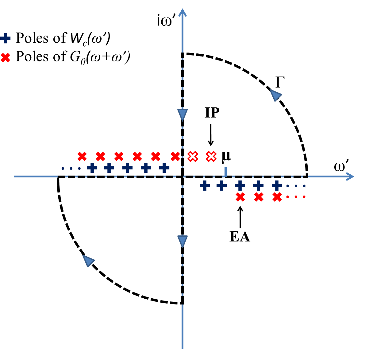
Fig 1. The contour deformation method for computing \(\Sigma^{c}\) over the contour \(\Gamma\). IP, \(\mu\) and EA represent ionization potential, chemical potential and electron affinity, respectively.
Basis set: Technical Execution of NAOs
The choice of basis set fully depends on the aim of calculation. The basis set could either be consisted of localized atomic orbitals or plane waves. In PyNAO, we have opted for the spatially localized basis sets for the following reasons:
First, it is widely accepted that simulation of materials containing localized states with d- or f-electrons with a finite set of basis functions such as Gaussian, Slater or numerical atomic orbitals (NAOs) are much more appropriate, while plane-wave basis sets in such conditions are extremely expensive [aryasetiawan1998gw].
Second, having established that plane-waves need periodic boundary conditions, the achievement of convergence for molecules placing in a supercell including the vacuum gap is computationally impractical [Freysoldt2008].
Linear combination of atomic orbital (LCAO) has been gaining importance in the recent decade not only for enhancing O(N) methods of the eigenvalue equation but also for forming more efficient basis sets with the high degree of accuracy for localized orbitals [Ozaki2004]. LCAO is an effective way to improve the applicability of electronic structure methods for evolving to the large systems. Therefore, to exploit these advantages, we performed LCAO for defining molecular orbitals and their products when single-particle wave functions in this framework could be expanded into coefficients (\(X_{a}^{i}\)) and atomic orbitals (\(\Phi^{a} (r)\)) as follows
here \(\Phi^{a} (r)\) could be decomposed into radial \(f^{a}(r)\) and spherical harmonic \(Y(\theta, \phi)\) segments being function of distance and direction of \(r\), respectively. For representing \(f^{a}(r)\), NAOs which are more flexible in this respect have been employed. In NAO, the accuracy and computational efficiency directly depend on the size, range, and radial shape of the atomic orbitals when accuracy can be maximized by optimizing the shape of the atomic orbitals [nao2001]. Particularly in gwa, the feasibility of using the product of NAOs is a very effective method [Foerster2011]. Fock operator is a sophisticated example that was recently noted by Koval P. et al. [koval2019GW]. To illustrate the performance of a spatially localized basis set made of NAOs, we turn our attention to the central elements of the gwa, i.e. full electron-hole matrix elements of the screened interaction \(I(\omega)\). Traditionally, It can be computed for occupied states \((n, m)\) by the following way
From the previous equations above one can summarize the \(GW\) correction in the form of bellow
In the \(G_0W_0\) method as implemented in PyNAO, \(E_{n, \sigma}\) will be iteratively corrected to achieve the convergency threshold. In this case, \(I^{nm\sigma}(i{\omega}')\) needs to be calculated once. Despite, this is the bottleneck of \(GW\) calculations and demands a huge amount of memory and processing. On the contrary, \(I^{nk\sigma} (z_k(E_{n,\sigma}))\) in the vicinity of the real frequency axis has to be repeated in each the iteration because of the dependency of \(z_k(E_n)\) on the QP eigenenergy \(E_n\). In PyNAO, we coded an iterative procedure using the advantages of NAOs to overcome the complexity of this level of calculations. So that by inserting LCAO and expansion of NAO’s products \((f^{a}(r)f^{b}(r))\) into the recent multi-centered integral, the latter equation will lead to an \(O(N^{4})\) operations.
At this point to have efficient performance in \(O(N^{3})\) scaling, a local basis of dominant products \((F^{\mu}(r))\) was constructed being related to NAO products via product vertex \((V_{\mu}^{ab})\) as follows [foerster2008]
This product vertex as a set of coefficients is a sparse matrix with nonzero elements if and only if all \(a, b, \mu\) belong to the same atom pair [talman1984numerical]. Consequently, \(I(\omega)\) takes the following tensorial form
where we introduced the product vertex between molecular orbitals as follows
here \(X_{a}^{\sigma n}\) and \(X_{b}^{\sigma m}\) are the corresponding coefficients of occupied states \((n, m)\) for each spin state \(\sigma\) where \(a\) and \(b\) represents which atomic orbitals are combined in the term. Similarly, the real space and tensorial equations of matrix elements of non-interacting irreducible polarizability \((P^{0})\) yields
Eventually, the correlation part of RPA-\(W\) in the tensorial format along real-frequency axes could be computed by the following equation
where \(\upsilon^{\mu \mu^{'}}\) represents the coulumb interaction and defined as \(\upsilon ^{\mu{\mu}'} = \int F^{\mu}(r)\frac{1}{\left|r-{r}'\right |}F^{{\mu}'}({r}')drd{r}'\). By the aim of this approach, the size of the basis will be decreased and helps to minimize memory usage for storing the whole matrix elements of \(W_{c}\) that will significantly affect the computational cost.
Examples
Starting calculations from SIESTA
After the SIESTA calculation is completed (see Runing DFT section),
one can use the stored data to compute \(G_0W_0\) correction.
The Python script needs to load the gw_iter class.
The loaded class can take the system label
as an argument in order to load the data from the prior SIESTA calculation.
We refer users to examples/S2_triplet directory to see example of input files for SIESTA and PyNAO that calculates \(G_0W_0\) energy levels for Disulfur molecule (\(S_2\)) as an open shell molecule with 2 unpaired valence electrons.
There are vast numbers of common arguments that can be kept in default values to start a trial calculation.
>>> from pynao import gw as gw_c
>>> import os
>>> dname = os.getcwd()
>>> gw = gw_c ( label = 'S2', cd = dname, rescf = True, magnetization = 2)
>>> gw.kernel_gw()
>>> gw.report()
Using Gaussian-based HF as implemented in PySCF
PyNAO was enabled to do \(G_0W_0\) correction on top of mean-field (so far
only HF) calculations done by PySCF code which performs a Gaussian type orbital
(GTO) basis set. A typical Python script to organize such a calculation for
\(O_2\) molecule is given below. In the first block of the script, we import
the PySCF’s objects gto and SCF as well as gw_iter class.
Then selected molecule with given coordinates of oxygen atoms and a desire Gaussian
basis set like Dunning’s basis cc-pVQZ was defined in the second block.
Here SCF.UHF does an unrestricted HF calculation and kernel computes the
corresponding energies, eigenfunctions, and so forth. The last block launches
\(G_0W_0\) class in the iterative scheme. At the end of this block
gw.kernel_gw_iter computes the \(G_0W_0\) corrections in
energies and report provides a plain-text report file including
QP spectra as well as mean-field energies.
>>> from pySCF import gto, SCF
>>> from pynao import gw\_iter
>>> mol = gto.M ( atom = '''O 0.0, 0.0, 0.622978 ; O 0.0, 0.0, -0.622978''', basis = 'ccpvqz' , spin = 2)
>>> mf = SCF.UHF (mol)
>>> mf.kernel()
>>> gw = gw_iter (mf = mf, gto = mol,
>>>   verbosity = 4,
>>>   niter_max_ev = 10, tol_ev = 1e-04,
>>>   nocc = 6 , nvrt = 10,
>>>   nff_ia = 28,
>>>   write_R = True,
>>>   limited_nbnd = False,
>>>   pass_dupl = False,
>>>   use_initial_guess_ite_solver = True,
>>>   SCF_kernel_conv_tol = 1.0e-6,
>>>   dtype = np.float32,
>>>   kmat_algo = 'sm0_sum',
>>>   gw_xvx_algo= "dp_sparse",
>>>   krylov_solver= "lgmres",
>>>   krylov_options= {"tol": 1.0e-3, "atol": 1.0e-3, "outer_k": 5})
>>> gw.kernel\_gw\_iter()
>>> gw.report()