Calculating Raman intensities
PyNAO can be used with the ASE vibrations module to calculate both
static and resonant intensities of the Raman vibration modes. It uses
the Placzek approximation implemented in ASE by Prof. M. Walter. When
using this module for your work, please cite
M. Walter and M. Moseler, Ab Initio Wavelength-Dependent Raman Spectra: Placzek Approximation and Beyond, J. Chem. Theory Comput. 2020, 16, 1, 576–586
In this example, we will calculate the Raman intensities of a CO2 molecule
Calculating the static Raman intensities
import numpy as np
from ase import Atoms
from ase.calculators.siesta import Siesta
from ase.calculators.siesta.siesta_lrtddft import RamanCalculatorInterface
from ase.vibrations.raman import StaticRamanCalculator
from ase.vibrations.placzek import PlaczekStatic
from ase.units import Ry, eV, Ha


CO2 = Atoms('CO2',
            positions=[[-0.009026, -0.020241, 0.026760],
                       [1.167544, 0.012723, 0.071808],
                       [-1.185592, -0.053316, -0.017945]],
            cell=[20, 20, 20])

# set-up the Siesta parameters
CO2.calc = Siesta(
      mesh_cutoff=250 * Ry,
      basis_set='DZP',
      pseudo_qualifier='gga',
      xc="PBE",
      energy_shift=(25 * 10**-3) * eV,
      fdf_arguments={
        'SCFMustConverge': False,
        'COOP.Write': True,
        'WriteDenchar': True,
        'PAO.BasisType': 'split',
        'DM.Tolerance': 1e-4,
        'DM.MixingWeight': 0.01,
        "MD.NumCGsteps": 0,
        "MD.MaxForceTol": (0.02, "eV/Ang"),
        'MaxSCFIterations': 10000,
        'DM.NumberPulay': 4,
        'XML.Write': True,
        "WriteCoorXmol": True,
        "DM.UseSaveDM": True,})

name = 'co2'
rm = StaticRamanCalculator(CO2, RamanCalculatorInterface, name=name, delta=0.011,
                           exkwargs=dict(label="siesta", jcutoff=7, iter_broadening=0.15,
                                         xc_code='LDA,PZ', tol_loc=1e-6, tol_biloc=1e-7,
                                         krylov_options={"tol": 1.0e-5, "atol": 1.0e-5}))

# save dipole moments from DFT calculation in order to get
# infrared intensities as well
rm.ir = True
rm.run()

pz = PlaczekStatic(CO2, name=name)
e_vib = pz.get_energies()
pz.summary()
Writing co2.eq.pckl, dipole moment = (-0.000052 0.000020 -0.000097)
Total number of iterations:  30
Writing co2.0x-.pckl, dipole moment = (-0.022999 -0.000500 -0.000805)
Total number of iterations:  30
Writing co2.0x+.pckl, dipole moment = (0.022946 0.000541 0.000611)
Total number of iterations:  30
Writing co2.0y-.pckl, dipole moment = (-0.000533 -0.004412 -0.000116)
Total number of iterations:  30
Writing co2.0y+.pckl, dipole moment = (0.000488 0.004502 -0.000077)
Total number of iterations:  30
Writing co2.0z-.pckl, dipole moment = (-0.000745 -0.000018 -0.004569)
Total number of iterations:  30
Writing co2.0z+.pckl, dipole moment = (0.000678 0.000041 0.004399)
Total number of iterations:  30
Writing co2.1x-.pckl, dipole moment = (0.011596 0.000281 0.000263)
Total number of iterations:  30
Writing co2.1x+.pckl, dipole moment = (-0.011393 -0.000232 -0.000437)
Total number of iterations:  30
Writing co2.1y-.pckl, dipole moment = (0.000231 0.002235 -0.000086)
Total number of iterations:  30
Writing co2.1y+.pckl, dipole moment = (-0.000311 -0.002257 -0.000108)
Total number of iterations:  30
Writing co2.1z-.pckl, dipole moment = (0.000287 0.000057 0.002160)
Total number of iterations:  30
Writing co2.1z+.pckl, dipole moment = (-0.000439 0.000007 -0.002387)
Total number of iterations:  30
Writing co2.2x-.pckl, dipole moment = (0.011357 0.000273 0.000251)
Total number of iterations:  30
Writing co2.2x+.pckl, dipole moment = (-0.011644 -0.000239 -0.000450)
Total number of iterations:  30
Writing co2.2y-.pckl, dipole moment = (0.000278 0.002249 -0.000085)
Total number of iterations:  30
Writing co2.2y+.pckl, dipole moment = (-0.000258 -0.002249 -0.000105)
Total number of iterations:  30
Writing co2.2z-.pckl, dipole moment = (0.000340 0.000061 0.002157)
Total number of iterations:  30
Writing co2.2z+.pckl, dipole moment = (-0.000338 0.000010 -0.002365)
Total number of iterations:  30
-------------------------------------
 Mode    Frequency        Intensity
  #    meV     cm^-1      [0.1A^4/amu]
-------------------------------------
  0    0.0       0.0       11.20
  1    0.0       0.0       12.43
  2   17.1     137.6        1.93
  3   20.7     166.9        6.13
  4   35.2     284.1        8.87
  5   76.7     618.4        0.07
  6   78.0     628.9        0.35
  7  173.3    1397.4      212.10
  8  309.9    2499.5        0.01
-------------------------------------
from ase.vibrations.infrared import InfraRed
# finite displacement for vibrations
ir = InfraRed(CO2, name=name)
ir.run()
ir.summary()
-------------------------------------
 Mode    Frequency        Intensity
  #    meV     cm^-1   (D/Å)^2 amu^-1
-------------------------------------
  0   34.2i    275.6i     0.0026
  1   29.7i    239.4i     0.0014
  2   17.1     137.6      0.0001
  3   20.7     166.9      0.0004
  4   35.2     284.1      0.0071
  5   76.7     618.4      0.5261
  6   78.0     628.9      0.5142
  7  173.3    1397.4      0.0008
  8  309.9    2499.5     13.9984
-------------------------------------
Zero-point energy: 0.355 eV
Static dipole moment: 0.001 D
Maximum force on atom in equilibrium: 1.0566 eV/Å
Summary
Let’s summarized our results for Infra-red and Raman intensities in a clear table.
Quantity |
Method |
1 bending |
2 stretching |
3 asymmetric streching |
|---|---|---|---|---|
\(\omega\) (cm\(^{-1}\)) |
exp |
667.00 |
1330.00 |
2349.00 |
ASE |
623.65 |
1397.40 |
2499.50 |
|
QE |
608.45 |
1271.13 |
2223.67 |
|
IR \((D/A)^{2}\) amu\(^{-1}\) |
ASE |
0.52 |
0.00 |
14.00 |
QE |
0.45 |
0.02 |
12.33 |
|
Raman (\(A^{4}\) amu\(^{-1}\)) |
ASE |
0.02 |
21.21 |
0.00 |
QE |
0.00 |
23.82 |
0.00 |
The intensities we calculated are given by the ASE rows, experimental values are given for the infra-red intensities values as well as Quantum Expresso calculations. More details can be found in Chapter 7 of M. Barbry PhD thesis.
Resonant Raman calculations
As explain in M. Walter paper, the Placzek is good enough to get the
resonant Raman intensities, for this one can pass the parameter omega
to the RamanCalculatorInterface object.
But first lets find the frequency we want to calculate for. In order to do this, we will calculate the polarizability of the CO2 molecule.
from ase.calculators.siesta.siesta_lrtddft import SiestaLRTDDFT

LRTDDFT = SiestaLRTDDFT(label="siesta", jcutoff=7, iter_broadening=0.15,
                        xc_code='LDA,PZ', tol_loc=1e-6, tol_biloc=1e-7,
                        krylov_options={"tol": 1.0e-5, "atol": 1.0e-5})

# run siesta
LRTDDFT.get_ground_state(CO2, mesh_cutoff=250 * Ry,
                         basis_set='DZP',
                         pseudo_qualifier='gga',
                         xc="PBE",
                         energy_shift=(25 * 10**-3) * eV,
                         fdf_arguments={
                            'SCFMustConverge': False,
                            'COOP.Write': True,
                            'WriteDenchar': True,
                            'PAO.BasisType': 'split',
                            'DM.Tolerance': 1e-4,
                            'DM.MixingWeight': 0.01,
                            "MD.NumCGsteps": 0,
                            "MD.MaxForceTol": (0.02, "eV/Ang"),
                            'MaxSCFIterations': 10000,
                            'DM.NumberPulay': 4,
                            'XML.Write': True,
                            "WriteCoorXmol": True,
                            "DM.UseSaveDM": True,})

# Get polarizability
freq = np.arange(0.0, 25.0, 0.5)
pmat = LRTDDFT.get_polarizability(freq)
Total number of iterations: 1756
import matplotlib.pyplot as plt

h = 9
w = 16*h/9
fig = plt.figure(1, figsize=(w, h))

iax = 1
for i in range(3):
    for j in range(3):
        ax = fig.add_subplot(3, 3, iax)

        ax.plot(freq, pmat[i, j, :].imag, linewidth=3)
        iax += 1

fig.tight_layout()
plt.show()
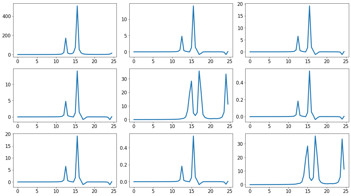
Let’s focus on the excitation around 15 eV
# Get polarizability
freq = np.arange(14.0, 16.0, 0.01)
pmat2 = LRTDDFT.get_polarizability(freq)
Total number of iterations: 8596
import matplotlib.pyplot as plt

h = 9
w = 16*h/9
fig = plt.figure(1, figsize=(w, h))

iax = 1
for i in range(3):
    for j in range(3):
        ax = fig.add_subplot(3, 3, iax)

        ax.plot(freq, pmat2[i, j, :].imag, linewidth=3)
        iax += 1

fig.tight_layout()
plt.show()
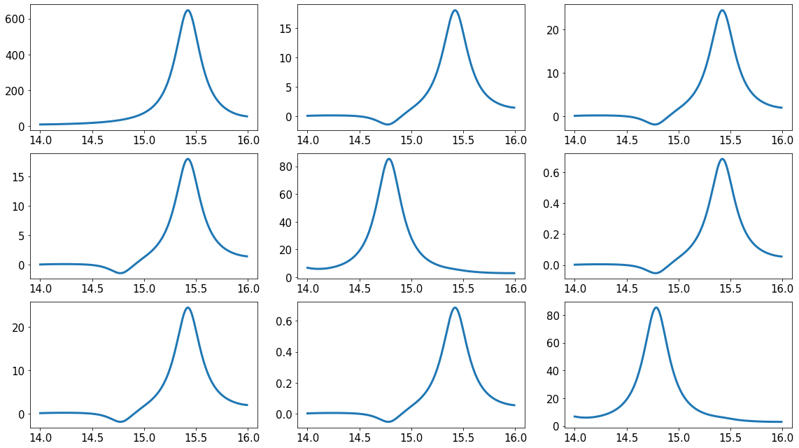
freq_max_int = freq[np.argmax(pmat2[2, 2, :])]
print("excitation frequency along zz is ", freq_max_int)
excitation frequency along zz is 14.639999999999986
name = 'co2-res'
rm = StaticRamanCalculator(CO2, RamanCalculatorInterface, name=name, delta=0.011,
                           exkwargs=dict(omega=freq_max_int, label="siesta", jcutoff=7, iter_broadening=0.15,
                                         xc_code='LDA,PZ', tol_loc=1e-6, tol_biloc=1e-7,
                                         krylov_options={"tol": 1.0e-5, "atol": 1.0e-5}, verbose=5))

# save dipole moments from DFT calculation in order to get
# infrared intensities as well
rm.ir = True
rm.run()

pz = PlaczekStatic(CO2, name=name)
e_vib = pz.get_energies()
pz.summary()
Writing co2-res.eq.pckl, dipole moment = (-0.000026 0.000020 -0.000117)
Total number of iterations:  45
Writing co2-res.0x-.pckl, dipole moment = (-0.023009 -0.000500 -0.000805)
Total number of iterations:  46
Writing co2-res.0x+.pckl, dipole moment = (0.022946 0.000541 0.000611)
Total number of iterations:  46
Writing co2-res.0y-.pckl, dipole moment = (-0.000533 -0.004412 -0.000116)
Total number of iterations:  49
Writing co2-res.0y+.pckl, dipole moment = (0.000488 0.004502 -0.000077)
Total number of iterations:  49
Writing co2-res.0z-.pckl, dipole moment = (-0.000745 -0.000018 -0.004569)
Total number of iterations:  49
Writing co2-res.0z+.pckl, dipole moment = (0.000678 0.000041 0.004399)
Total number of iterations:  49
Writing co2-res.1x-.pckl, dipole moment = (0.011596 0.000281 0.000263)
Total number of iterations:  47
Writing co2-res.1x+.pckl, dipole moment = (-0.011393 -0.000232 -0.000437)
Total number of iterations:  46
Writing co2-res.1y-.pckl, dipole moment = (0.000231 0.002235 -0.000086)
Total number of iterations:  49
Writing co2-res.1y+.pckl, dipole moment = (-0.000311 -0.002257 -0.000108)
Total number of iterations:  49
Writing co2-res.1z-.pckl, dipole moment = (0.000287 0.000057 0.002160)
Total number of iterations:  49
Writing co2-res.1z+.pckl, dipole moment = (-0.000439 0.000007 -0.002387)
Total number of iterations:  49
Writing co2-res.2x-.pckl, dipole moment = (0.011357 0.000273 0.000251)
Total number of iterations:  46
Writing co2-res.2x+.pckl, dipole moment = (-0.011644 -0.000239 -0.000450)
Total number of iterations:  47
Writing co2-res.2y-.pckl, dipole moment = (0.000278 0.002249 -0.000085)
Total number of iterations:  49
Writing co2-res.2y+.pckl, dipole moment = (-0.000258 -0.002249 -0.000105)
Total number of iterations:  49
Writing co2-res.2z-.pckl, dipole moment = (0.000340 0.000061 0.002157)
Total number of iterations:  49
Writing co2-res.2z+.pckl, dipole moment = (-0.000338 0.000010 -0.002365)
Total number of iterations:  49
-------------------------------------
 Mode    Frequency        Intensity
  #    meV     cm^-1      [100A^4/amu]
-------------------------------------
  0    0.0       0.0        0.32
  1    0.0       0.0        0.40
  2   17.1     137.6        0.35
  3   20.7     166.9        0.20
  4   35.2     284.1        0.25
  5   76.7     618.4        0.02
  6   78.0     628.9        0.02
  7  173.3    1397.4      318.36
  8  309.9    2499.3        0.02
-------------------------------------
res = 100*318.36
static = 0.1*212.10
print(static, res, res/static)
21.21 31836.0 1500.9900990099009
Raman intensities enhancement
Let’s analyse the enhancement of the resonant Raman intensity compared to the static one for the mode at \(\omega = 1397.4\) cm\(^{-1}\). The intensities are (taking into account the scaling factor in the summary)
static: \(I_{sta} = 21.21\) A\(^{4}\)/amu
resonant: \(I_{res} = 31836.0\) A\(^{4}\)/amu
Leading to an enhancement of around 1500